In computational complexity theory, big O notation is often used to describe how the size of the input data affects an algorithm's usage of computational resources (usually running time or memory). It is also called Big Oh notation, Landau notation, and asymptotic notation. Big O notation is also used in many other scientific and mathematical fields to provide similar estimations.
The symbol O is used to describe an asymptotic upper bound for the magnitude of a function in terms of another, usually simpler, function. There are also other symbols o, Ω, ω, and Θ for various other upper, lower, and tight bounds. Informally, the O notation is commonly employed to describe an asymptotic tight bound, but tight bounds are more formally and precisely denoted by the Θ (capital theta) symbol as described below. This distiction between upper and tight bounds is useful, and sometimes critical, and most computer scientists would urge distinguishing the usage of O and Θ, but in some other fields the Θ notation is not commonly known.

Usage
In a way to be made precise below, O(f(x)) denotes the collection of functions g(x) – viewed as a function of variable x – that exhibit a growth that is limited to that of f(x) in some respect. The traditional notation for stating that g(x) belongs to this collection is:

This is an anomalous and exceptional use of the equals sign in mathematics, as the above statement is not an equation. It is improper to conclude from g(x) = O(f(x)) and h(x) = O(f(x)) that g(x) and h(x) are equal. One way to think of this, is to consider "= O" one symbol here. To avoid the anomalous use, some authors prefer to write instead:

without difference in meaning.
The common arithmetic operations are often extended to the class concept. For example, h(x) + O(f(x)) denotes the collection of functions having the growth of h(x) plus a part whose growth is limited to that of f(x). Thus,

expresses the same as

Another anomaly of the notation, although less exceptional, is that it does not make explicit which variable is the function argument, which may need to be inferred from the context if several variables are involved. The following two right-hand side big O notations have dramatically different meanings:


The first case states that f(m) exhibits polynomial growth, while the second, assuming m > 1, states that g(n) exhibits exponential growth. So as to avoid all possible confusion, some authors use the notation

meaning the same as what is denoted by others as

A final anomaly is that the notation does not make clear "where" the function growth is to be considered; infinitesimally near some point, or in the neighbourhood of infinity. This is in contrast with the usual notation for limits. A similar notational device as for limits would resolve both this and the preceding anomaly, but is not in use.

Equals or member-of and other notational anomalies
Big O notation is useful when analyzing algorithms for efficiency. For example, the time (or the number of steps) it takes to complete a problem of size n might be found to be T(n) = 4n² - 2n + 2.
As n grows large, the n² term will come to dominate, so that all other terms can be neglected—for instance when n = 500, the term 4n² is 1000 times as large as the 2n term. Ignoring the latter would have negligible effect on the expression's value for most purposes.
Further, the coefficients become irrelevant as well if we compare to any other order of expression, such as an expression containing a term n³ or n². Even if T(n) = 1,000,000n², if U(n) = n³, the latter will always exceed the former once n grows larger than 1,000,000 (T(1,000,000) = 1,000,000³ = U(1,000,000)).
So the big O notation captures what remains: we write

(read as "big o of n squared") and say that the algorithm has order of n² time complexity.

Infinite asymptotics
Big O can also be used to describe the error term in an approximation to a mathematical function. For example,

expresses the fact that the error, the difference , is smaller in absolute value than some constant times when x is close enough to 0.

Infinitesimal asymptotics
Suppose f(x) and g(x) are two functions defined on some subset of the real numbers. We say

if and only if

The notation can also be used to describe the behavior of f near some real number a: we say

if and only if

If g(x) is non-zero for values of x sufficiently close to a, both of these definitions can be unified using the limit superior:

if and only if

In mathematics, both asymptotic behaviours near ∞ and near a are considered. In computational complexity theory, only asymptotics near ∞ are used; furthermore, only positive functions are considered, so the absolute value bars may be left out.

Example
The statement "f(x) is O(g(x))" as defined above is usually written as f(x) = O(g(x)). This is a slight abuse of notation; equality of two functions is not asserted, and it cannot be since the property of being O(g(x)) is not symmetric:
.
There is also a second reason why that notation is not precise. The symbol f(x) means the value of the function f for the argument x. Hence the symbol of the function is f and not f(x).
For these reasons, some authors prefer set notation and write , thinking of as the set of all functions dominated by g.
In more complex usage, O( ) can appear in different places in an equation, even several times on each side. For example, the following are true for



The meaning of such statements is as follows: for any functions which satisfy each O( ) on the left side, there are some functions satisfying each O( ) on the right side, such that substituting all these functions into the equation makes the two sides equal. For example, the third equation above means: "For any function f(n)=O(1), there is some function g(n)=O(e=g(n)." In terms of the "set notation" above, the meaning is that the class of functions represented by the left side is a subset of the class of functions represented by the right side.

Matters of notation
Here is a list of classes of functions that are commonly encountered when analyzing algorithms. All of these are as n increases to infinity. The slower-growing functions are listed first. c is an arbitrary constant.
Not as common, but even larger growth is possible, such as the single-valued version of the Ackermann function, A(n,n). Conversely, extremely slowly-growing functions such as the inverse of this function, often denoted α(n), are possible. Although unbounded, these functions are often regarded as being constant factors for all practical purposes.

Common orders of functions
If a function f(n) can be written as a finite sum of other functions, then the fastest growing one determines the order of f(n). For example

In particular, if a function may be bounded by a polynomial in n, then as n tends to infinity, one may disregard lower-order terms of the polynomial.
O(n (unless, of course, c=1).

Properties



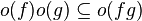
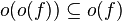
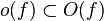
Product



Sum



Multiplication by a constant
Big O is the most commonly used asymptotic notation for comparing functions, although in many cases Big O may be replaced with Θ for asymptotically tighter bounds (Theta, see below). Here, we define some related notations in terms of "big O":

Related asymptotic notations
The relation is read as "f(x) is little-oh of g(x)". Intuitively, it means that g(x) grows much faster than f(x). It assumes that f and g are both functions of one variable. Formally, it states that the limit of f(x) / g(x) is zero, as x approaches infinity.
For example,
Little-o notation is common in mathematics but rarer in computer science. In computer science the variable (and function value) is most often a natural number. In math, the variable and function values are often real numbers. The following properties can be useful:
As with big O notation, the statement "f(x) is o(g(x))" is usually written as f(x) = o(g(x)), which is a slight abuse of notation.






(and thus the above properties apply with most combinations of o and O). Little-o notation
For more details on other notations go to: Asymptotic Growth of Functions

Other related notations
Big O (and little o, and Ω...) can also be used with multiple variables. For example, the statement

asserts that there exist constants C and N such that

where g(n,m) is defined by
f(n,m) = n + g(n,m).
To avoid ambiguity, the running variable should always be specified: the statement

is quite different from


Multiple variables
It is often useful to bound the running time of graph algorithms. Unlike most other computational problems, for a graph G = (V, E) there are two relevant parameters describing the size of the input: the number |V| of vertices in the graph and the number |E| of edges in the graph. Inside asymptotic notation (and only there), it is common to use the symbols V and E, when someone really means |V| and |E|. We adopt this convention here to simplify asymptotic functions and make them easily readable. The symbols V and E are never used inside asymptotic notation with their literal meaning, so this abuse of notation does not risk ambiguity. For example O(E + VlogV) means for a suitable metric of graphs. Another common convention—referring to the values |V| and |E| by the names n and m, respectively—sidesteps this ambiguity.

Generalizations and related usages

Asymptotic Growth of Functions: Presentation and definition of all notations.
Asymptotic expansion: Approximation of functions generalizing Taylor's formula.
Asymptotically optimal: A phrase frequently used to describe an algorithm that has an upper bound asymptotically within a constant of a lower bound for the problem
Hardy notation: A different asymptotic notation
Limit superior and limit inferior: An explanation of some of the limit notation used in this article
Nachbin's theorem: A precise way of bounding complex analytic functions so that the domain of convergence of integral transforms can be stated.